# ruff: noqa: E402
Estimating parameters of an anharmonic oscillator#
The anharnomic oscillator can be modelled by a non-linear partial differential equation as described in section 6.3.4 of the book Fundamentals of Algorithms and Data Assimilation by Mark Asch, Marc Bocquet and Maëlle Nodet.
The discrete two-parameter model is:
with initial conditions \(x_0 = 0\) and \(x_1 = 1\).
In other words we have the following recurrence relationship:
\(x_{k+1} = \omega^2 x_{k} - \lambda^2 x_{k}^3 + 2 x_{k} - x_{k-1}\)
The state vector can be written as:
so that \(\mathbf{u}_{k+1} = \mathcal{M}_{k+1}(\mathbf{u}_k)\).
import numpy as np
from matplotlib import pyplot as plt
from scipy import stats

import iterative_ensemble_smoother as ies

rng = np.random.default_rng(12345)

plt.rcParams["figure.figsize"] = [8, 3]
def plot_result(A, response_x_axis, title=None):
    """Plot the anharmonic oscillator, as well as marginal
    and joint distributions for the parameters."""

    responses = forward_model(A, response_x_axis)

    fig, axes = plt.subplots(1, 2 + len(A), figsize=(9, 2.25))
    if title:
        fig.suptitle(title)

    axes[0].plot(response_x_axis, responses, color="black", alpha=0.1)
    for ax, param, label in zip(axes[1:], A, ["omega", "lambda"]):
        ax.hist(param, bins="fd")
        ax.set_xlabel(label)

    axes[-1].scatter(A[0, :], A[1, :], s=5)

    fig.tight_layout()
    plt.show()
Setup#
def generate_observations(K):
    """Run the model with true parameters, then generate observations."""
    # Evaluate using true parameter values on a fine grid with K sample points
    x = simulate_anharmonic(omega=3.5e-2, lmbda=3e-4, K=K)

    # Generate observations every `nobs` steps
    nobs = 50
    # Generate observation points [0, 50, 100, 150, ...] when `nobs` = 50
    observation_x_axis = np.arange(K // nobs) * nobs

    # Generate noisy observations, with value at least 5
    observation_errors = np.maximum(5, 0.2 * np.abs(x[observation_x_axis]))
    observation_values = rng.normal(loc=x[observation_x_axis], scale=observation_errors)

    return observation_values, observation_errors, observation_x_axis


def simulate_anharmonic(omega, lmbda, K):
    """Evaluate the anharmonic oscillator."""
    x = np.zeros(K)
    x[0] = 0
    x[1] = 1

    # Looping from 2 because we have initial conditions at k=0 and k=1.
    for k in range(2, K):
        x[k] = x[k - 1] * (2 + omega**2 - lmbda**2 * x[k - 1] ** 2) - x[k - 2]

    return x


def forward_model(A, response_x_axis):
    """Evaluate on each column (ensemble realization)."""
    return np.vstack(
        [simulate_anharmonic(*params, K=len(response_x_axis)) for params in A.T]
    ).T


response_x_axis = range(2500)
observation_values, observation_errors, observation_x_axis = generate_observations(
    len(response_x_axis)
)
Plot observations#
fig, ax = plt.subplots(figsize=(8, 3))
ax.set_title("Anharmonic Oscillator")
ax.plot(
    np.arange(2500),
    simulate_anharmonic(omega=3.5e-2, lmbda=3e-4, K=2500),
    label="Truth",
    color="black",
)

ax.scatter(observation_x_axis, observation_values, label="Observations")

fig.tight_layout()
plt.legend()
plt.show()

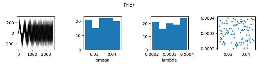
Create and plot prior#
This section shows a “trick” for working with non-normal priors.
Let \(g\) be the forward model, so that \(y = g(x)\). Assume for instance that \(x\) must be a positive parameter. If so, then we can for instance use an exponential prior on \(x\). But if we use samples from an exponential prior directly in an ensemble smoother, there is no guarantee that the posterior samples will be positive.
The trick is to sample \(x \sim \mathcal{N}(0, 1)\), then define a function \(f\) that maps from standard normal to the exponential distribution. This function can be constructed by first mapping from standard normal to the interval \([0, 1)\) using the CDF, then mapping to exponential using the quantile function (inverse CDF) of the exponential distribution.
In summary:
We send \(x \sim \mathcal{N}(0, 1)\) into the ensemble smoother as before
We use the composite function \(g(f(x))\) as our forward model, instead of \(g(x)\)
When we plot the prior and posterior, we plot \(f(x)\) instead of \(x\) directly
# Create Uniform prior distributions
realizations = 100
PRIORS = [stats.uniform(loc=0.025, scale=0.02), stats.uniform(loc=0.0002, scale=0.0002)]
def prior_to_standard_normal(A):
    """Map prior to U(0, 1), then use inverse of CDF to map to N(0, 1)."""
    return np.vstack(
        [stats.norm().ppf(prior.cdf(A_param)) for (A_param, prior) in zip(A, PRIORS)]
    )


def standard_normal_to_prior(A):
    """Reverse mapping."""
    return np.vstack(
        [prior.ppf(stats.norm().cdf(A_param)) for (A_param, prior) in zip(A, PRIORS)]
    )


# verify that mappings are invertible
A_uniform = np.vstack([prior.rvs(realizations) for prior in PRIORS])
assert np.allclose(
    standard_normal_to_prior(prior_to_standard_normal(A_uniform)), A_uniform
)
assert np.allclose(
    prior_to_standard_normal(standard_normal_to_prior(A_uniform)), A_uniform
)
# Create a standard normal prior and plot it in transformed space
A = rng.standard_normal(size=(2, realizations))
plot_result(standard_normal_to_prior(A), response_x_axis)

A single update step#
plot_result(standard_normal_to_prior(A), response_x_axis)

# The forward model is composed with the transformation from N(0, 1) to uniform priors
responses_before = forward_model(standard_normal_to_prior(A), response_x_axis)
Y = responses_before[observation_x_axis]

# Run smoother for one step
smoother = ies.SIES(
    parameters=A,
    covariance=observation_errors**2,
    observations=observation_values,
    seed=42,
)

new_A = smoother.sies_iteration(Y, step_length=1.0)


plot_result(standard_normal_to_prior(new_A), response_x_axis)

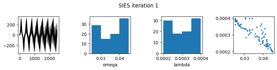
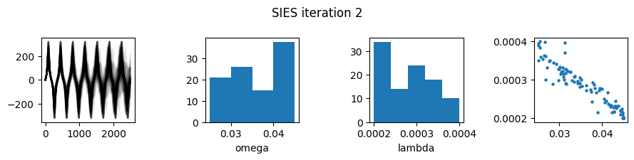
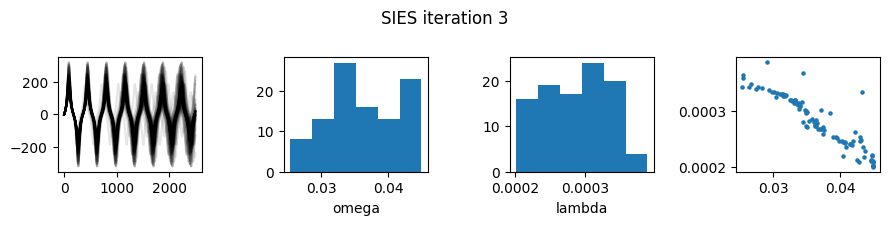
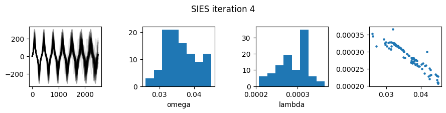
Iterative smoother#
from iterative_ensemble_smoother.utils import steplength_exponential


def iterative_smoother(A):
    A_current = np.copy(A)
    iterations = 4
    smoother = ies.SIES(
        parameters=A,
        covariance=observation_errors**2,
        observations=observation_values,
        seed=42,
    )

    plot_result(
        standard_normal_to_prior(A_current),
        response_x_axis,
        title="Prior",
    )

    for iteration in range(iterations):
        responses_before = forward_model(
            standard_normal_to_prior(A_current), response_x_axis
        )

        Y = responses_before[observation_x_axis]

        A_current = smoother.sies_iteration(
            Y, step_length=steplength_exponential(iteration + 1)
        )

        plot_result(
            standard_normal_to_prior(A_current),
            response_x_axis,
            title=f"SIES iteration {iteration+1}",
        )


iterative_smoother(A)
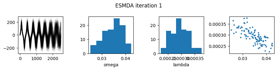
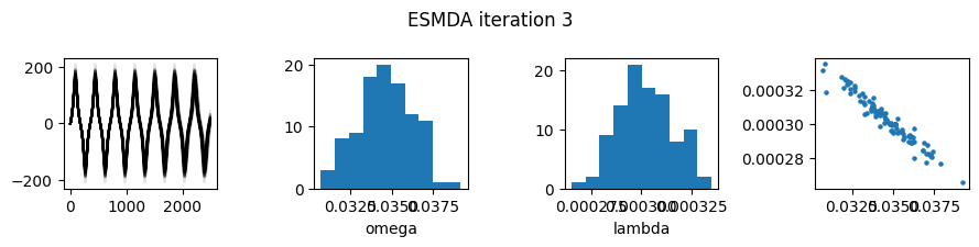
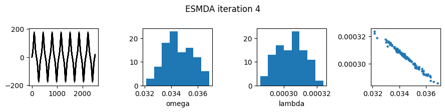
ES-MDA (Ensemble Smoother - Multiple Data Assimilation)#
smoother = ies.ESMDA(
    # If a 1D array is passed, it is interpreted
    # as the diagonal of the covariance matrix.
    covariance=observation_errors**2,
    observations=observation_values,
    # The inflation factors used in ESMDA
    # They are scaled so that sum_i alpha_i^-1 = 1
    alpha=np.array([8, 4, 2, 1]),
    seed=42,
)


A_current = np.copy(A)

plot_result(standard_normal_to_prior(A_current), response_x_axis, title="Prior")

for iteration in range(smoother.num_assimilations()):
    # Evaluate the model
    responses_before = forward_model(
        standard_normal_to_prior(A_current), response_x_axis
    )
    Y = responses_before[observation_x_axis]

    # Assimilate data
    A_current = smoother.assimilate(A_current, Y)

    # Plot
    plot_result(
        standard_normal_to_prior(A_current),
        response_x_axis,
        title=f"ESMDA iteration {iteration+1}",
    )